Analysis Report

library(aphantasiaEmotions)
#> Welcome to aphantasiaEmotions.
library(patchwork)

Sample description

By dataset

all_data |>
  dplyr::group_by(study) |>
  dplyr::reframe(
    Language = unique(lang),
    N = paste0(
      dplyr::n(),
      " (",
      sum(gender == "female", na.rm = TRUE),
      " F, ",
      sum(gender == "other", na.rm = TRUE),
      " O)"
    ),
    M_age = mean(age, na.rm = TRUE),
    SD_age = sd(age, na.rm = TRUE),
    min_age = min(age, na.rm = TRUE),
    max_age = max(age, na.rm = TRUE),
  ) |>
  knitr::kable(digits = 2)

study	Language	N	M_age	SD_age	min_age	max_age
burns	en	192 (122 F, 3 O)	38.69	11.44	18	86
monzel	en	105 (74 F, 0 O)	27.87	9.29	18	59
mas	fr	123 (110 F, 0 O)	19.78	1.15	18	24
ruby	fr	225 (180 F, 3 O)	35.96	16.07	10	82
kvamme	en	833 (426 F, 5 O)	40.45	13.44	18	83

By VVIQ group

all_data |>
  dplyr::group_by(vviq_group_4) |>
  dplyr::reframe(
    N = paste0(
      dplyr::n(),
      " (",
      sum(gender == "female", na.rm = TRUE),
      " F, ",
      sum(gender == "other", na.rm = TRUE),
      " O)"
    ),
    M_age = mean(age, na.rm = TRUE),
    SD_age = sd(age, na.rm = TRUE),
    min_age = min(age, na.rm = TRUE),
    max_age = max(age, na.rm = TRUE),
    M_vviq = mean(vviq, na.rm = TRUE),
    SD_vviq = sd(vviq, na.rm = TRUE)
  ) |>
  dplyr::rename("VVIQ group" = 1) |> 
  knitr::kable(digits = 2)

VVIQ group	N	M_age	SD_age	min_age	max_age	M_vviq	SD_vviq
aphantasia	147 (102 F, 5 O)	40.27	12.90	19	86	16.00	0.00
hypophantasia	141 (87 F, 1 O)	36.40	12.21	17	64	24.33	4.61
typical	1115 (675 F, 4 O)	36.34	14.47	10	82	55.33	10.05
hyperphantasia	75 (48 F, 1 O)	40.48	14.95	16	83	77.31	1.90

By dataset, VVIQ and TAS-20 (alexithymia) group

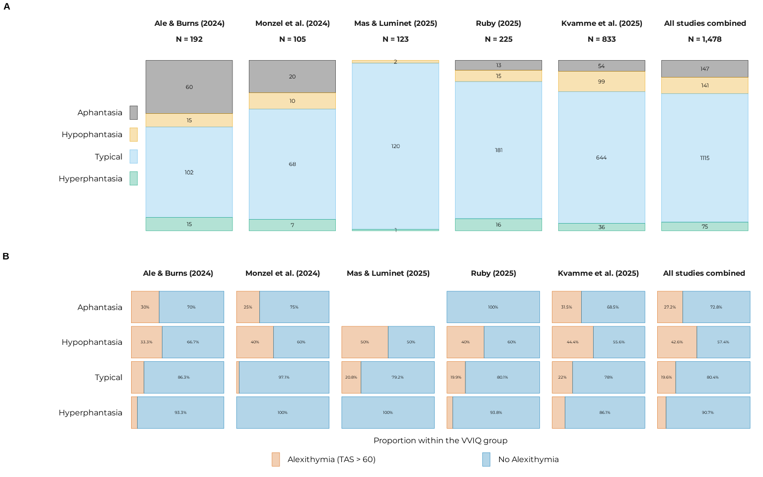
p_counts <-
  all_data |>
  dplyr::bind_rows(all_data |> dplyr::mutate(study = "total")) |>
  dplyr::mutate(
    study = factor(
      study,
      levels = c("burns", "monzel", "mas", "ruby", "kvamme", "total")
    )
  ) |>
  plot_vviq_group_proportions(vviq_group_4, base_size = 12, prop_txt_size = 3)

p_props <-
  all_data |>
  summarise_aph_and_alexi(vviq_group_4) |>
  plot_alexithymia_proportions(
    vviq_group_4,
    ncol = 6,
    base_size = 12,
    prop_txt_size = 2
  )

ggpubr::ggarrange(
  p_counts,
  p_props,
  ncol = 1,
  heights = c(1.1, 1),
  labels = "AUTO",
  font.label = list(size = 14, face = "bold")
)

Modelling

Bayesian setup

Bayesian models were fitted using the brms::brm() function from the brms package (Bürkner, 2017) through a custom wrapper, fit_brms_model(), that sets several default options for us. 24000 post-warmup iterations were spread across all available CPU for parallel processing¹, with 2000 additional warmup iterations per chain. A fixed seed was used for reproducibility. Regularising priors were used to improve convergence and avoid overfitting. A weakly informative normal prior with mean 0 and standard deviation 20 was used on the fixed effects to improve the default flat priors of brms. Default weakly informative priors from brms were used for other model parameters. The adequacy of these priors were assessed using a prior predictive check, which is presented below. To avoid having to refit the models each time the vignette is built and improve reproducibility, fitted models are saved in the models/ folder (or inst/models/ in the source code on GitHub) and loaded in the R chunks.

After model fit, we checked model performance using posterior predictive checks with the performance::check_predictions() function to ensure that the models were able to reproduce the data well.

We tested our hypotheses on linear models with marginal contrasts between VVIQ groups. This task was performed with functions from the marginaleffects package. We used the marginaleffects::avg_comparisons() function to compute contrasts and a custom report_rope() wrapper (around marginaleffects::posterior_draws(), bayestestR::rope_range() and bayestestR::p_direction()) to summarise their posterior distributions. We computed the probability of direction (PD) of the contrasts and the proportions of their posterior distributions below, inside or above a region of practical equivalence to the null (ROPE) (see Makowski et al., 2019).

The dynamics of non-linear models was analysed using the modelbased::estimate_slopes() function to compute the variation of the outcome variable per unit change in VVIQ across its range. We summarised the evidence for positive or negative slopes using a custom check_slope_evidence() function that computes the PD and ROPE proportions of the slope estimates.

The setup of marginaleffects options and model priors is done in the chunk below.

options("marginaleffects_safe" = FALSE)
draws <- seq(1, 4000, 1) # To limit draws that will be used for marginaleffects

priors <- c(brms::prior(normal(0, 20), class = "b"))
refit  <- "never"

Prior predictive check were performed to ensure that the priors set on the models were adequate. This was done by fitting a model with the same structure as the planned analyses but sampling only from the prior distributions. The posterior predictive distributions of this prior-only model were then plotted to check that they covered a reasonable range of values.

lm_prior <-
  fit_brms_model(
    formula = tas ~ vviq_group_4,
    data = all_data,
    prior = priors,
    sample_prior = "only",
    file_refit = refit,
    file = system.file("models/lm_prior.rds", package = "aphantasiaEmotions")
  )

performance::check_predictions(lm_prior, draw_ids = 1:12) |>
  plot() +
  ggplot2::labs(title = "Prior Predictive Check") +
  theme_pdf(base_size = 12)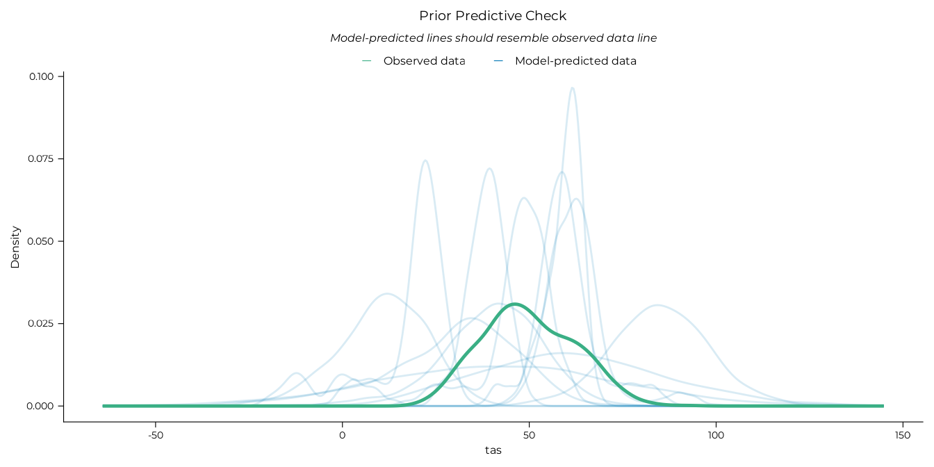

Here we go!

Analysis of total TAS-20 scores

Linear categorical model

# Group model
lm_tot <-
  fit_brms_model(
    formula = tas ~ vviq_group_4,
    data = all_data,
    prior = priors,
    file_refit = refit,
    file = system.file("models/lm_tot.rds", package = "aphantasiaEmotions")
  )

# Posterior predictive check
performance::check_predictions(lm_tot, draw_ids = 1:12) |>
  plot() +
  theme_pdf(base_size = 12)
#> Ignoring unknown labels:
#> • size : ""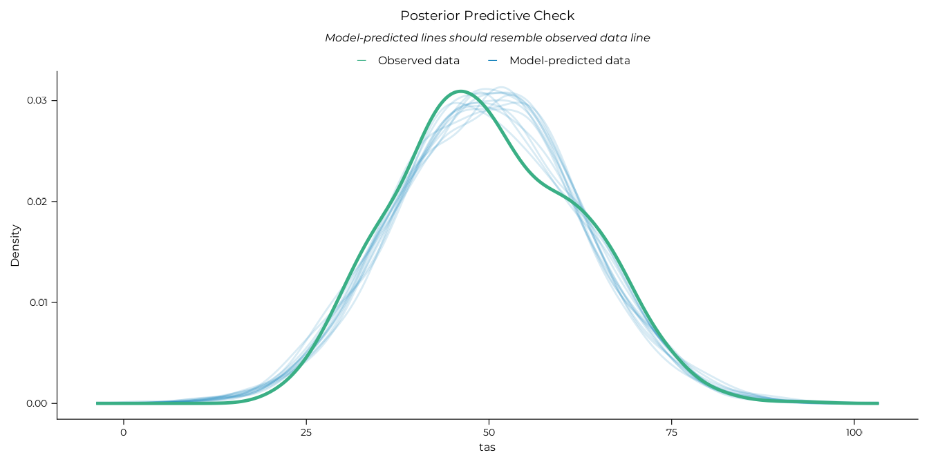

contrasts_tot <-
  marginaleffects::comparisons(
    lm_tot,
    variables = list("vviq_group_4" = "pairwise"),
    draw_ids = draws
  )

report_rope(contrasts_tot, contrast) |> knitr::kable()

contrast	Estimate	95% CI	d	PD	Below ROPE	Inside ROPE	Above ROPE
hyperphantasia - aphantasia	-8.387	[-11.741, -5.042]	0.67	1.000	1.000	0.00	0.000
hyperphantasia - hypophantasia	-14.595	[-17.923, -11.115]	1.17	1.000	1.000	0.00	0.000
hyperphantasia - typical	-7.000	[-9.795, -4.196]	0.56	1.000	1.000	0.00	0.000
hypophantasia - aphantasia	6.168	[3.302, 8.993]	0.49	1.000	0.000	0.00	1.000
typical - aphantasia	-1.373	[-3.439, 0.623]	0.11	0.903	0.544	0.45	0.005
typical - hypophantasia	-7.551	[-9.683, -5.343]	0.60	1.000	1.000	0.00	0.000

p_contr_tot <-
  plot_posterior_contrasts(
    contrasts_tot,
    lm_tot,
    base_size = 12,
    rope_txt = 3,
    dot_size = 1,
    x_lab = "Effect size (TAS score difference)",
    axis_relative_x = 0.7
  )

# Group plot
p_tot <-
  plot_group_violins(
    tas ~ vviq_group_4,
    y_lab = "Total TAS Score",
    base_size = 12
  ) +
  plot_alexithymia_cutoff(txt_size = 2, txt_x = 1.4, label = "Alexithymia") +
  scale_discrete_aphantasia() +
  scale_x_aphantasia(add = c(0.4, 0.7))

plot(p_tot + p_contr_tot)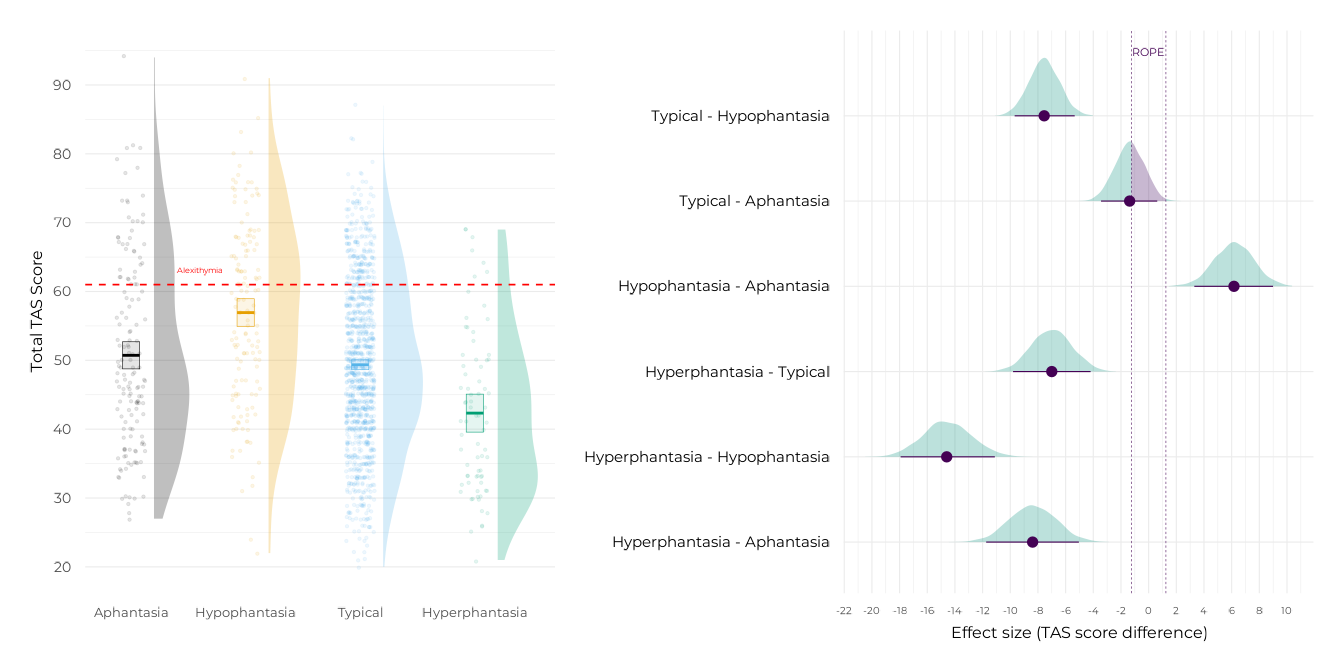

Nonlinear continuous model

gam_tot <-
  fit_brms_model(
    formula = tas ~ s(vviq),
    data = all_data,
    prior = priors,
    file_refit = refit,
    file = system.file("models/gam_tot.rds", package = "aphantasiaEmotions")
  )

# Posterior predictive check
performance::check_predictions(gam_tot, draw_ids = 1:12) |>
  plot() +
  theme_pdf(base_size = 12)
#> Ignoring unknown labels:
#> • size : ""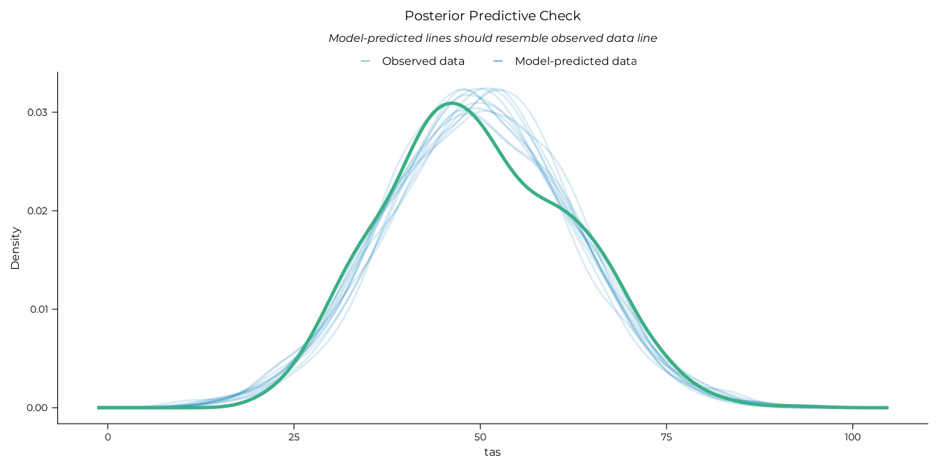

slopes_tot <-
  modelbased::estimate_slopes(
    gam_tot,
    trend = "vviq",
    by = "vviq",
    length = 75,
    rope_ci = 1
  )

check_slope_evidence(slopes_tot) |> knitr::kable()

VVIQ	Median	CI	PD	Evidence
16	0.477	[0.107, 0.977]	0.996	Non null
17	0.476	[0.108, 0.971]	0.996	Non null
18	0.470	[0.111, 0.95]	0.996	Non null
19	0.458	[0.114, 0.91]	0.997	Non null
20	0.436	[0.115, 0.851]	0.997	Non null
21	0.404	[0.112, 0.778]	0.997	Non null
22	0.360	[0.096, 0.707]	0.997	Non null
23	0.305	[0.067, 0.63]	0.995	Non null
24	0.243	[0.018, 0.552]	0.984	Non null
25	0.178	[-0.055, 0.469]	0.938	Uncertain
26	0.114	[-0.144, 0.381]	0.829	Uncertain
27	0.050	[-0.241, 0.291]	0.659	Uncertain
28	-0.012	[-0.338, 0.212]	0.540	Uncertain
29	-0.068	[-0.432, 0.148]	0.714	Uncertain
30	-0.117	[-0.521, 0.103]	0.828	Uncertain
31	-0.158	[-0.591, 0.072]	0.895	Uncertain
32	-0.188	[-0.636, 0.047]	0.931	Uncertain
33	-0.208	[-0.65, 0.03]	0.953	Uncertain
34	-0.219	[-0.634, 0.015]	0.965	Uncertain
35	-0.221	[-0.591, 0.006]	0.972	Non null
36	-0.216	[-0.543, 0]	0.975	Non null
37	-0.207	[-0.49, 0.011]	0.969	Uncertain
38	-0.196	[-0.452, 0.037]	0.956	Uncertain
39	-0.187	[-0.428, 0.073]	0.936	Uncertain
40	-0.181	[-0.415, 0.107]	0.917	Uncertain
41	-0.181	[-0.407, 0.129]	0.909	Uncertain
42	-0.186	[-0.403, 0.125]	0.910	Uncertain
43	-0.196	[-0.408, 0.099]	0.924	Uncertain
44	-0.211	[-0.414, 0.063]	0.945	Uncertain
45	-0.230	[-0.427, 0.021]	0.967	Uncertain
46	-0.251	[-0.457, -0.021]	0.982	Non null
47	-0.272	[-0.488, -0.053]	0.990	Non null
48	-0.290	[-0.521, -0.081]	0.995	Non null
49	-0.307	[-0.545, -0.108]	0.998	Non null
50	-0.320	[-0.56, -0.129]	0.999	Non null
51	-0.329	[-0.562, -0.141]	1.000	Non null
52	-0.332	[-0.556, -0.145]	0.999	Non null
53	-0.331	[-0.549, -0.139]	0.999	Non null
54	-0.326	[-0.541, -0.128]	0.999	Non null
55	-0.321	[-0.53, -0.112]	0.997	Non null
56	-0.313	[-0.515, -0.099]	0.996	Non null
57	-0.306	[-0.499, -0.09]	0.995	Non null
58	-0.300	[-0.488, -0.086]	0.995	Non null
59	-0.297	[-0.484, -0.081]	0.995	Non null
60	-0.297	[-0.486, -0.08]	0.994	Non null
61	-0.299	[-0.495, -0.077]	0.994	Non null
62	-0.303	[-0.508, -0.08]	0.994	Non null
63	-0.309	[-0.519, -0.088]	0.995	Non null
64	-0.316	[-0.527, -0.1]	0.996	Non null
65	-0.323	[-0.533, -0.114]	0.998	Non null
66	-0.329	[-0.539, -0.125]	0.998	Non null
67	-0.334	[-0.553, -0.124]	0.998	Non null
68	-0.337	[-0.571, -0.115]	0.997	Non null
69	-0.336	[-0.585, -0.102]	0.996	Non null
70	-0.335	[-0.594, -0.091]	0.995	Non null
71	-0.334	[-0.599, -0.083]	0.994	Non null
72	-0.330	[-0.597, -0.076]	0.994	Non null
73	-0.327	[-0.602, -0.071]	0.993	Non null
74	-0.323	[-0.615, -0.054]	0.990	Non null
75	-0.321	[-0.643, -0.025]	0.983	Non null
76	-0.317	[-0.674, 0.009]	0.972	Non null
77	-0.314	[-0.706, 0.042]	0.960	Uncertain
78	-0.312	[-0.733, 0.066]	0.950	Uncertain
79	-0.312	[-0.747, 0.078]	0.945	Uncertain
80	-0.312	[-0.751, 0.081]	0.943	Uncertain

p_slopes_tot <-
  plot_gam_slopes(
    slopes_tot,
    .f_groups = dplyr::case_when(
      vviq <= 24 ~ 1,
      vviq <= 34 ~ 2,
      vviq <= 36 ~ 3,
      vviq <= 45 ~ 4,
      vviq <= 76 ~ 5,
      vviq <= 80 ~ 6
    ),
    y_lab = "TAS variation per unit change in VVIQ",
    base_size = 12
  )

p_gam_tot <-
  plot_gam_means(
    gam_tot,
    y_lab = "Total TAS score",
    legend_relative = 0.85,
    base_size = 12
  ) +
  plot_coloured_subjects(
    x = all_data$vviq,
    y = all_data$tas,
    size = 1
  ) +
  plot_alexithymia_cutoff(txt_x = 26, label = "Alexithymia") +
  scale_discrete_aphantasia() +
  scale_x_vviq()

plot(p_gam_tot + p_slopes_tot)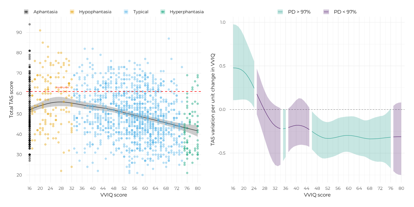

Analysis of TAS-20 sub-scale scores

Linear categorical models

# Subscale group models
lm_dif <-
  fit_brms_model(
    formula = tas_identify ~ vviq_group_4,
    data = all_data,
    prior = priors,
    file_refit = refit,
    file = system.file("models/lm_dif.rds", package = "aphantasiaEmotions")
  )

lm_ddf <-
  fit_brms_model(
    formula = tas_describe ~ vviq_group_4,
    data = all_data,
    prior = priors,
    file_refit = refit,
    file = system.file("models/lm_ddf.rds", package = "aphantasiaEmotions")
  )

lm_eot <-
  fit_brms_model(
    formula = tas_external ~ vviq_group_4,
    data = all_data,
    prior = priors,
    file_refit = refit,
    file = system.file("models/lm_eot.rds", package = "aphantasiaEmotions")
  )

# Posterior predictive checks
pp_dif_lm <-
  performance::check_predictions(lm_dif, draw_ids = 1:12) |>
  plot() +
  theme_pdf(base_size = 12)

pp_ddf_lm <-
  performance::check_predictions(lm_ddf, draw_ids = 1:12) |>
  plot() +
  theme_pdf(base_size = 12)

pp_eot_lm <-
  performance::check_predictions(lm_eot, draw_ids = 1:12) |>
  plot() +
  theme_pdf(base_size = 12)

plot(pp_dif_lm / pp_ddf_lm / pp_eot_lm)
#> Ignoring unknown labels:
#> • size : ""
#> Ignoring unknown labels:
#> • size : ""
#> Ignoring unknown labels:
#> • size : ""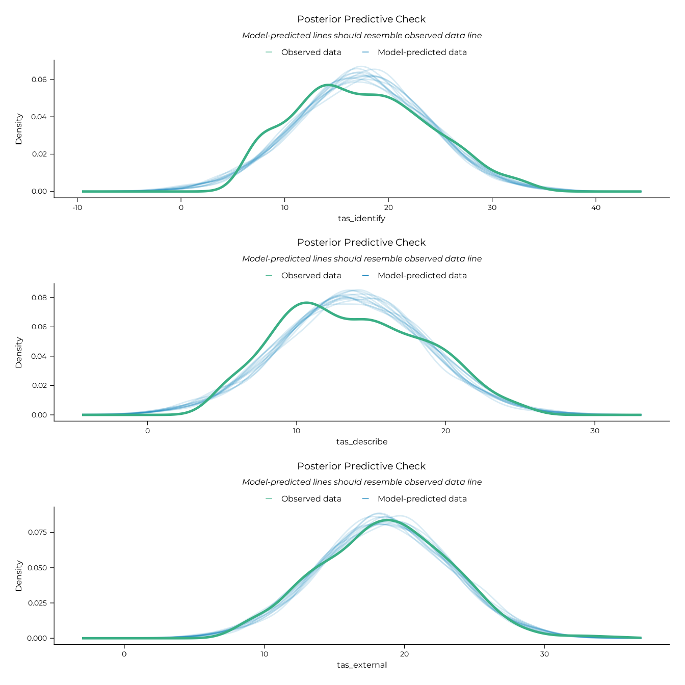

contrasts_dif <-
  marginaleffects::comparisons(
    lm_dif,
    variables = list("vviq_group_4" = "pairwise"),
    draw_ids = draws
  )

report_rope(contrasts_dif, contrast) |> knitr::kable()

contrast	Estimate	95% CI	d	PD	Below ROPE	Inside ROPE	Above ROPE
hyperphantasia - aphantasia	-3.399	[-5.143, -1.69]	0.53	1.000	0.999	0.001	0.000
hyperphantasia - hypophantasia	-6.199	[-7.908, -4.419]	0.97	1.000	1.000	0.000	0.000
hyperphantasia - typical	-2.850	[-4.251, -1.403]	0.45	1.000	1.000	0.000	0.000
hypophantasia - aphantasia	2.790	[1.344, 4.231]	0.44	1.000	0.000	0.002	0.999
typical - aphantasia	-0.556	[-1.605, 0.462]	0.09	0.847	0.445	0.543	0.012
typical - hypophantasia	-3.351	[-4.48, -2.225]	0.53	1.000	1.000	0.000	0.000

contrasts_ddf <-
  marginaleffects::comparisons(
    lm_ddf,
    variables = list("vviq_group_4" = "pairwise"),
    draw_ids = draws
  )

report_rope(contrasts_ddf, contrast) |> knitr::kable()

contrast	Estimate	95% CI	d	PD	Below ROPE	Inside ROPE	Above ROPE
hyperphantasia - aphantasia	-2.841	[-4.128, -1.526]	0.59	1.000	1.000	0.000	0.000
hyperphantasia - hypophantasia	-5.028	[-6.328, -3.773]	1.05	1.000	1.000	0.000	0.000
hyperphantasia - typical	-2.379	[-3.442, -1.268]	0.50	1.000	1.000	0.000	0.000
hypophantasia - aphantasia	2.198	[1.097, 3.254]	0.46	1.000	0.000	0.002	0.998
typical - aphantasia	-0.461	[-1.278, 0.32]	0.10	0.877	0.485	0.506	0.009
typical - hypophantasia	-2.658	[-3.484, -1.84]	0.55	1.000	1.000	0.000	0.000

contrasts_eot <-
  marginaleffects::comparisons(
    lm_eot,
    variables = list("vviq_group_4" = "pairwise"),
    draw_ids = draws
  )

report_rope(contrasts_eot, contrast) |> knitr::kable()

contrast	Estimate	95% CI	d	PD	Below ROPE	Inside ROPE	Above ROPE
hyperphantasia - aphantasia	-2.117	[-3.404, -0.829]	0.45	1.000	0.995	0.005	0.000
hyperphantasia - hypophantasia	-3.332	[-4.679, -2.005]	0.72	1.000	1.000	0.000	0.000
hyperphantasia - typical	-1.798	[-2.922, -0.691]	0.39	1.000	0.992	0.009	0.000
hypophantasia - aphantasia	1.220	[0.207, 2.295]	0.26	0.990	0.001	0.076	0.923
typical - aphantasia	-0.323	[-1.107, 0.476]	0.07	0.785	0.368	0.605	0.028
typical - hypophantasia	-1.555	[-2.388, -0.705]	0.33	1.000	0.995	0.005	0.000

# Subscale group plots
p_dif <-
  plot_group_violins(
    tas_identify ~ vviq_group_4,
    y_lab = "TAS DIF Score",
    base_size = 12
  ) +
  scale_discrete_aphantasia() +
  scale_x_aphantasia(add = c(0.4, 0.7))
p_ddf <-
  plot_group_violins(
    tas_describe ~ vviq_group_4,
    y_lab = "TAS DDF Score",
    base_size = 12
  ) +
  scale_discrete_aphantasia() +
  scale_x_aphantasia(add = c(0.4, 0.7))
p_eot <-
  plot_group_violins(
    tas_external ~ vviq_group_4,
    y_lab = "TAS EOT Score",
    base_size = 12
  ) +
  scale_discrete_aphantasia() +
  scale_x_aphantasia(add = c(0.4, 0.7))

# Subscale contrast plots
p_dif_contr <-
  plot_posterior_contrasts(
    contrasts_dif,
    lm_dif,
    xlab = "Effect size (DIF score difference)",
    base_size = 12,
    dot_size = 1,
    axis_relative_x = 0.7
  )
p_ddf_contr <-
  plot_posterior_contrasts(
    contrasts_ddf,
    lm_ddf,
    xlab = "Effect size (DDF score difference)",
    base_size = 12,
    dot_size = 1,
    axis_relative_x = 0.7
  )
p_eot_contr <-
  plot_posterior_contrasts(
    contrasts_eot,
    lm_eot,
    xlab = "Effect size (EOT score difference)",
    base_size = 12,
    dot_size = 1,
    axis_relative_x = 0.7
  )

((p_dif + p_dif_contr) + plot_layout(tag_level = "new")) /
  ((p_ddf + p_ddf_contr) + plot_layout(tag_level = "new")) /
  ((p_eot + p_eot_contr) + plot_layout(tag_level = "new")) +
  plot_annotation(tag_levels = c("A", "1")) &
  ggplot2::theme(plot.tag = ggplot2::element_text(size = 10, face = "bold"))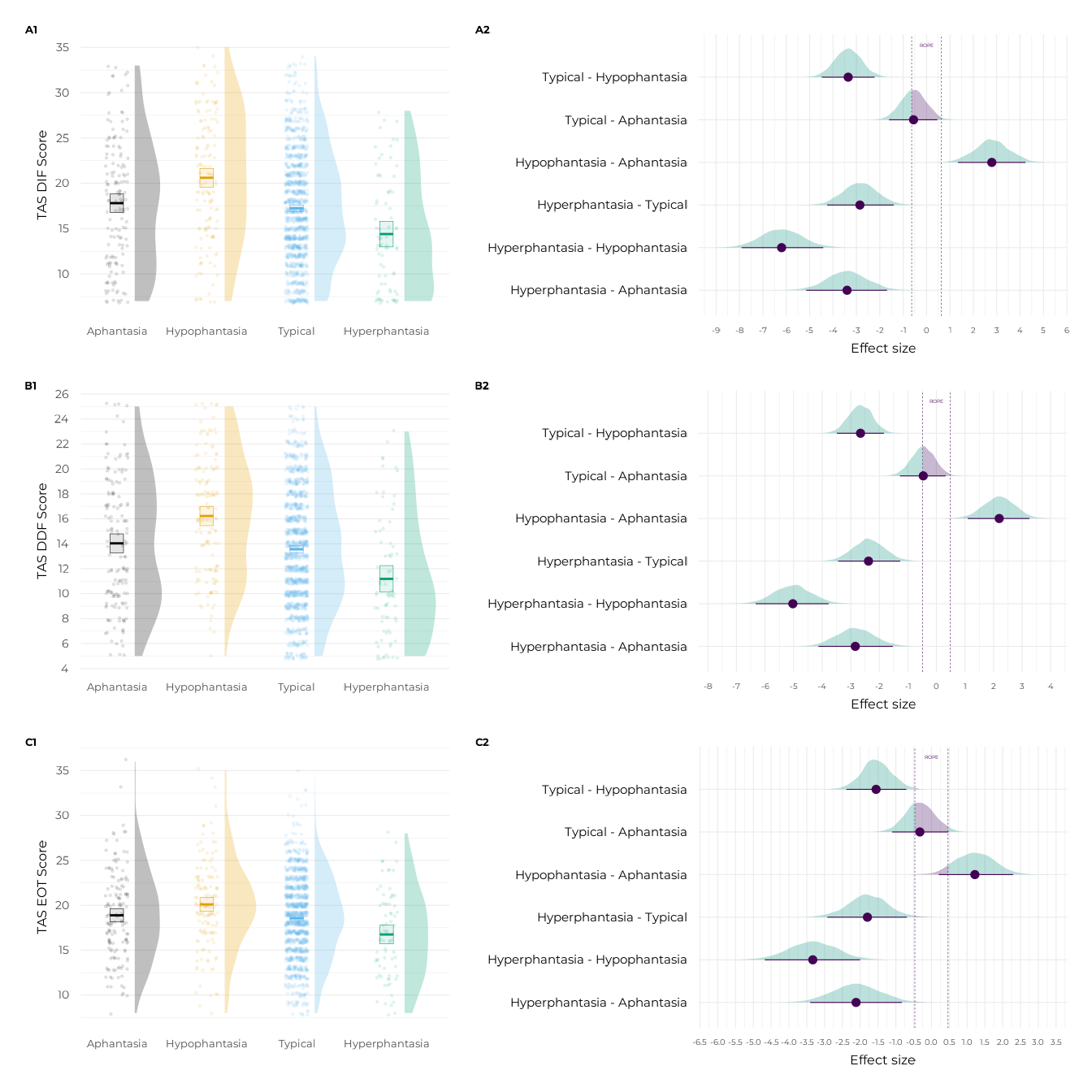

Nonlinear continuous models

# Subscale GAM models
gam_dif <-
  fit_brms_model(
    formula = tas_identify ~ s(vviq),
    data = all_data,
    prior = priors,
    file_refit = refit,
    file = system.file("models/gam_dif.rds", package = "aphantasiaEmotions")
  )

gam_ddf <-
  fit_brms_model(
    formula = tas_describe ~ s(vviq),
    data = all_data,
    prior = priors,
    file_refit = refit,
    file = system.file("models/gam_ddf.rds", package = "aphantasiaEmotions")
  )

gam_eot <-
  fit_brms_model(
    formula = tas_external ~ s(vviq),
    data = all_data,
    prior = priors,
    file_refit = refit,
    file = system.file("models/gam_eot.rds", package = "aphantasiaEmotions")
  )

# Posterior predictive checks
pp_dif_gam <-
  performance::check_predictions(gam_dif, draw_ids = 1:12) |>
  plot() +
  theme_pdf(base_size = 12)

pp_ddf_gam <-
  performance::check_predictions(gam_ddf, draw_ids = 1:12) |>
  plot() +
  theme_pdf(base_size = 12)

pp_eot_gam <-
  performance::check_predictions(gam_eot, draw_ids = 1:12) |>
  plot() +
  theme_pdf(base_size = 12)

plot(pp_dif_gam / pp_ddf_gam / pp_eot_gam)
#> Ignoring unknown labels:
#> • size : ""
#> Ignoring unknown labels:
#> • size : ""
#> Ignoring unknown labels:
#> • size : ""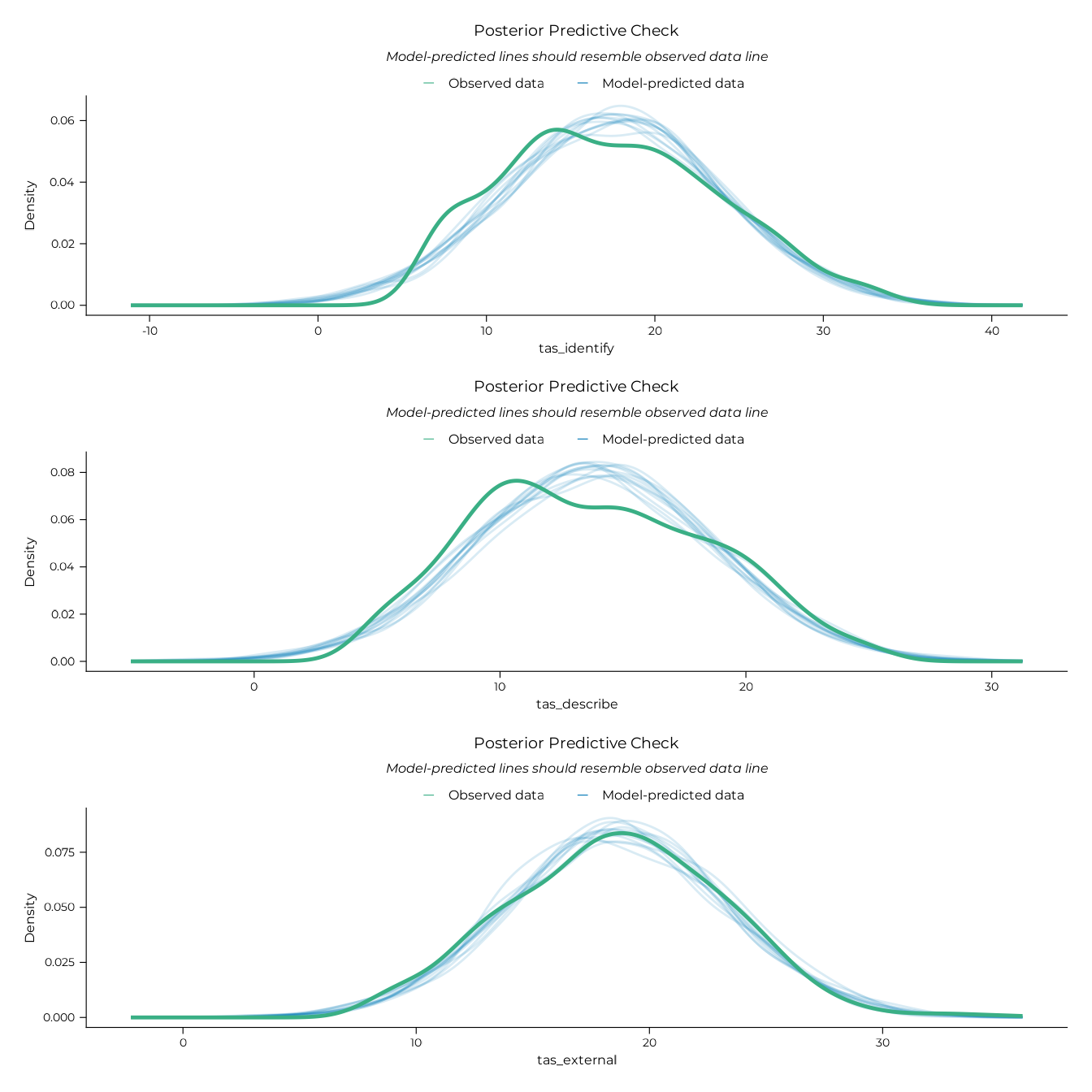

slopes_dif <-
  modelbased::estimate_slopes(gam_dif, trend = "vviq", by = "vviq", length = 75)

check_slope_evidence(slopes_dif) |> knitr::kable()

VVIQ	Median	CI	PD	Evidence
16	0.251	[0.012, 0.562]	0.982	Non null
17	0.250	[0.013, 0.559]	0.983	Non null
18	0.248	[0.015, 0.546]	0.984	Non null
19	0.243	[0.017, 0.519]	0.985	Non null
20	0.231	[0.019, 0.481]	0.986	Non null
21	0.214	[0.018, 0.437]	0.986	Non null
22	0.188	[0.013, 0.393]	0.984	Non null
23	0.154	[0.003, 0.354]	0.977	Non null
24	0.115	[-0.018, 0.31]	0.950	Uncertain
25	0.074	[-0.057, 0.262]	0.863	Uncertain
26	0.033	[-0.114, 0.201]	0.691	Uncertain
27	-0.006	[-0.177, 0.138]	0.534	Uncertain
28	-0.044	[-0.242, 0.084]	0.744	Uncertain
29	-0.083	[-0.304, 0.045]	0.879	Uncertain
30	-0.118	[-0.365, 0.02]	0.942	Uncertain
31	-0.146	[-0.416, 0.004]	0.970	Uncertain
32	-0.166	[-0.452, -0.007]	0.981	Non null
33	-0.177	[-0.466, -0.014]	0.987	Non null
34	-0.180	[-0.457, -0.018]	0.990	Non null
35	-0.176	[-0.426, -0.02]	0.992	Non null
36	-0.164	[-0.385, -0.021]	0.992	Non null
37	-0.146	[-0.336, -0.017]	0.988	Non null
38	-0.124	[-0.291, 0]	0.975	Non null
39	-0.101	[-0.252, 0.034]	0.941	Uncertain
40	-0.081	[-0.221, 0.076]	0.883	Uncertain
41	-0.065	[-0.196, 0.115]	0.814	Uncertain
42	-0.052	[-0.176, 0.143]	0.750	Uncertain
43	-0.042	[-0.159, 0.155]	0.704	Uncertain
44	-0.035	[-0.148, 0.155]	0.675	Uncertain
45	-0.034	[-0.144, 0.146]	0.671	Uncertain
46	-0.036	[-0.146, 0.132]	0.692	Uncertain
47	-0.043	[-0.152, 0.116]	0.730	Uncertain
48	-0.051	[-0.163, 0.094]	0.778	Uncertain
49	-0.060	[-0.176, 0.073]	0.830	Uncertain
50	-0.069	[-0.188, 0.053]	0.881	Uncertain
51	-0.078	[-0.199, 0.036]	0.917	Uncertain
52	-0.085	[-0.208, 0.024]	0.941	Uncertain
53	-0.091	[-0.216, 0.018]	0.953	Uncertain
54	-0.096	[-0.224, 0.016]	0.957	Uncertain
55	-0.099	[-0.225, 0.015]	0.958	Uncertain
56	-0.101	[-0.223, 0.014]	0.959	Uncertain
57	-0.104	[-0.219, 0.013]	0.962	Uncertain
58	-0.106	[-0.217, 0.009]	0.966	Uncertain
59	-0.108	[-0.217, 0.007]	0.969	Uncertain
60	-0.112	[-0.221, 0.006]	0.970	Uncertain
61	-0.116	[-0.23, 0.005]	0.970	Non null
62	-0.122	[-0.239, 0.003]	0.972	Non null
63	-0.128	[-0.249, -0.003]	0.977	Non null
64	-0.134	[-0.255, -0.013]	0.984	Non null
65	-0.141	[-0.262, -0.025]	0.990	Non null
66	-0.148	[-0.271, -0.035]	0.992	Non null
67	-0.154	[-0.284, -0.037]	0.993	Non null
68	-0.158	[-0.296, -0.035]	0.992	Non null
69	-0.162	[-0.308, -0.032]	0.991	Non null
70	-0.164	[-0.318, -0.029]	0.990	Non null
71	-0.165	[-0.319, -0.028]	0.989	Non null
72	-0.166	[-0.319, -0.028]	0.988	Non null
73	-0.165	[-0.321, -0.022]	0.986	Non null
74	-0.163	[-0.334, -0.008]	0.979	Non null
75	-0.161	[-0.355, 0.015]	0.965	Uncertain
76	-0.159	[-0.379, 0.041]	0.946	Uncertain
77	-0.157	[-0.402, 0.066]	0.926	Uncertain
78	-0.156	[-0.419, 0.085]	0.910	Uncertain
79	-0.156	[-0.429, 0.097]	0.902	Uncertain
80	-0.156	[-0.431, 0.1]	0.900	Uncertain

slopes_ddf <-
  modelbased::estimate_slopes(gam_ddf, trend = "vviq", by = "vviq", length = 75)

check_slope_evidence(slopes_ddf) |> knitr::kable()

VVIQ	Median	CI	PD	Evidence
16	0.169	[0.014, 0.405]	0.986	Non null
17	0.168	[0.014, 0.401]	0.986	Non null
18	0.165	[0.014, 0.389]	0.987	Non null
19	0.159	[0.016, 0.367]	0.988	Non null
20	0.150	[0.017, 0.333]	0.989	Non null
21	0.136	[0.016, 0.296]	0.989	Non null
22	0.118	[0.013, 0.256]	0.988	Non null
23	0.095	[0.004, 0.218]	0.980	Non null
24	0.070	[-0.016, 0.184]	0.945	Uncertain
25	0.046	[-0.05, 0.152]	0.847	Uncertain
26	0.023	[-0.093, 0.12]	0.694	Uncertain
27	0.002	[-0.133, 0.091]	0.516	Uncertain
28	-0.018	[-0.167, 0.066]	0.651	Uncertain
29	-0.036	[-0.195, 0.048]	0.773	Uncertain
30	-0.050	[-0.219, 0.035]	0.854	Uncertain
31	-0.061	[-0.238, 0.026]	0.903	Uncertain
32	-0.069	[-0.251, 0.019]	0.929	Uncertain
33	-0.073	[-0.247, 0.014]	0.946	Uncertain
34	-0.075	[-0.236, 0.011]	0.954	Uncertain
35	-0.074	[-0.217, 0.009]	0.958	Uncertain
36	-0.072	[-0.196, 0.011]	0.957	Uncertain
37	-0.069	[-0.177, 0.018]	0.947	Uncertain
38	-0.066	[-0.164, 0.028]	0.930	Uncertain
39	-0.063	[-0.156, 0.043]	0.910	Uncertain
40	-0.063	[-0.152, 0.054]	0.891	Uncertain
41	-0.063	[-0.15, 0.058]	0.883	Uncertain
42	-0.065	[-0.15, 0.055]	0.888	Uncertain
43	-0.069	[-0.15, 0.048]	0.907	Uncertain
44	-0.074	[-0.153, 0.035]	0.929	Uncertain
45	-0.081	[-0.161, 0.019]	0.953	Uncertain
46	-0.089	[-0.169, 0.004]	0.972	Non null
47	-0.097	[-0.182, -0.01]	0.983	Non null
48	-0.104	[-0.196, -0.022]	0.992	Non null
49	-0.110	[-0.207, -0.035]	0.996	Non null
50	-0.115	[-0.213, -0.044]	0.999	Non null
51	-0.119	[-0.215, -0.05]	0.999	Non null
52	-0.120	[-0.216, -0.052]	0.999	Non null
53	-0.119	[-0.213, -0.049]	0.999	Non null
54	-0.117	[-0.209, -0.045]	0.999	Non null
55	-0.113	[-0.204, -0.039]	0.997	Non null
56	-0.108	[-0.195, -0.032]	0.995	Non null
57	-0.103	[-0.182, -0.025]	0.993	Non null
58	-0.098	[-0.173, -0.017]	0.989	Non null
59	-0.093	[-0.164, -0.01]	0.984	Non null
60	-0.090	[-0.161, -0.002]	0.977	Non null
61	-0.087	[-0.161, 0.004]	0.970	Uncertain
62	-0.085	[-0.161, 0.01]	0.964	Uncertain
63	-0.085	[-0.162, 0.01]	0.964	Uncertain
64	-0.085	[-0.163, 0.007]	0.968	Uncertain
65	-0.087	[-0.163, 0.001]	0.974	Non null
66	-0.089	[-0.167, -0.003]	0.978	Non null
67	-0.091	[-0.173, -0.005]	0.980	Non null
68	-0.094	[-0.182, -0.002]	0.978	Non null
69	-0.096	[-0.191, -0.001]	0.976	Non null
70	-0.097	[-0.198, -0.001]	0.976	Non null
71	-0.099	[-0.202, 0]	0.975	Non null
72	-0.099	[-0.206, 0.002]	0.973	Non null
73	-0.099	[-0.21, 0.007]	0.967	Uncertain
74	-0.099	[-0.221, 0.017]	0.952	Uncertain
75	-0.098	[-0.236, 0.033]	0.930	Uncertain
76	-0.097	[-0.254, 0.052]	0.908	Uncertain
77	-0.096	[-0.269, 0.069]	0.888	Uncertain
78	-0.096	[-0.28, 0.08]	0.873	Uncertain
79	-0.095	[-0.286, 0.086]	0.865	Uncertain
80	-0.095	[-0.288, 0.089]	0.862	Uncertain

slopes_eot <-
  modelbased::estimate_slopes(gam_eot, trend = "vviq", by = "vviq", length = 75)

check_slope_evidence(slopes_eot) |> knitr::kable()

VVIQ	Median	CI	PD	Evidence
16	0.105	[-0.011, 0.26]	0.961	Uncertain
17	0.105	[-0.011, 0.258]	0.962	Uncertain
18	0.104	[-0.008, 0.25]	0.964	Uncertain
19	0.101	[-0.004, 0.237]	0.970	Uncertain
20	0.097	[0.001, 0.218]	0.976	Non null
21	0.092	[0.004, 0.197]	0.980	Non null
22	0.084	[0.004, 0.177]	0.982	Non null
23	0.076	[-0.001, 0.163]	0.974	Non null
24	0.067	[-0.011, 0.152]	0.956	Uncertain
25	0.058	[-0.025, 0.143]	0.927	Uncertain
26	0.049	[-0.038, 0.134]	0.889	Uncertain
27	0.041	[-0.05, 0.124]	0.850	Uncertain
28	0.034	[-0.057, 0.114]	0.808	Uncertain
29	0.027	[-0.062, 0.104]	0.767	Uncertain
30	0.022	[-0.066, 0.098]	0.720	Uncertain
31	0.017	[-0.069, 0.095]	0.673	Uncertain
32	0.012	[-0.073, 0.094]	0.623	Uncertain
33	0.007	[-0.075, 0.094]	0.579	Uncertain
34	0.003	[-0.077, 0.093]	0.529	Uncertain
35	-0.002	[-0.08, 0.09]	0.524	Uncertain
36	-0.008	[-0.083, 0.084]	0.587	Uncertain
37	-0.016	[-0.089, 0.078]	0.657	Uncertain
38	-0.024	[-0.096, 0.069]	0.727	Uncertain
39	-0.033	[-0.107, 0.059]	0.795	Uncertain
40	-0.042	[-0.118, 0.046]	0.860	Uncertain
41	-0.053	[-0.131, 0.031]	0.913	Uncertain
42	-0.065	[-0.143, 0.014]	0.955	Uncertain
43	-0.076	[-0.155, -0.004]	0.979	Non null
44	-0.087	[-0.168, -0.019]	0.992	Non null
45	-0.097	[-0.182, -0.032]	0.997	Non null
46	-0.106	[-0.194, -0.042]	0.999	Non null
47	-0.114	[-0.205, -0.048]	0.999	Non null
48	-0.119	[-0.213, -0.054]	1.000	Non null
49	-0.123	[-0.215, -0.058]	1.000	Non null
50	-0.125	[-0.213, -0.061]	1.000	Non null
51	-0.124	[-0.207, -0.062]	1.000	Non null
52	-0.122	[-0.2, -0.061]	1.000	Non null
53	-0.120	[-0.193, -0.056]	1.000	Non null
54	-0.116	[-0.187, -0.049]	0.999	Non null
55	-0.112	[-0.18, -0.042]	0.997	Non null
56	-0.107	[-0.174, -0.035]	0.996	Non null
57	-0.104	[-0.169, -0.03]	0.995	Non null
58	-0.101	[-0.164, -0.028]	0.994	Non null
59	-0.099	[-0.162, -0.026]	0.994	Non null
60	-0.098	[-0.163, -0.025]	0.993	Non null
61	-0.097	[-0.164, -0.024]	0.994	Non null
62	-0.097	[-0.168, -0.024]	0.994	Non null
63	-0.097	[-0.171, -0.027]	0.995	Non null
64	-0.097	[-0.173, -0.029]	0.996	Non null
65	-0.097	[-0.174, -0.03]	0.997	Non null
66	-0.095	[-0.173, -0.028]	0.996	Non null
67	-0.092	[-0.173, -0.023]	0.994	Non null
68	-0.088	[-0.173, -0.015]	0.989	Non null
69	-0.083	[-0.17, -0.003]	0.979	Non null
70	-0.076	[-0.164, 0.009]	0.961	Uncertain
71	-0.069	[-0.155, 0.022]	0.936	Uncertain
72	-0.061	[-0.148, 0.036]	0.897	Uncertain
73	-0.052	[-0.143, 0.055]	0.842	Uncertain
74	-0.043	[-0.142, 0.078]	0.777	Uncertain
75	-0.037	[-0.146, 0.103]	0.718	Uncertain
76	-0.031	[-0.15, 0.13]	0.669	Uncertain
77	-0.027	[-0.156, 0.152]	0.638	Uncertain
78	-0.025	[-0.16, 0.167]	0.619	Uncertain
79	-0.023	[-0.163, 0.175]	0.610	Uncertain
80	-0.023	[-0.164, 0.177]	0.608	Uncertain

p_slopes_dif <-
  plot_gam_slopes(
    slopes_dif,
    .f_groups = dplyr::case_when(
      vviq <= 23 ~ 1,
      vviq <= 31 ~ 2,
      vviq <= 38 ~ 3,
      vviq <= 60 ~ 4,
      vviq <= 74 ~ 5,
      vviq <= 80 ~ 6
    ),
    y_lab = "DIF variation per unit change in VVIQ",
    axis.title.y = ggplot2::element_text(size = 9),
    base_size = 12
  )

p_slopes_ddf <-
  plot_gam_slopes(
    slopes_ddf,
    .f_groups = dplyr::case_when(
      vviq <= 23 ~ 1,
      vviq <= 45 ~ 2,
      vviq <= 60 ~ 3,
      vviq <= 64 ~ 4,
      vviq <= 72 ~ 5,
      vviq <= 80 ~ 6
    ),
    y_lab = "DDF variation per unit change in VVIQ",
    legend.position = "none",
    axis.title.y = ggplot2::element_text(size = 9),
    base_size = 12
  )

p_slopes_eot <-
  plot_gam_slopes(
    slopes_eot,
    .f_groups = dplyr::case_when(
      vviq <= 19 ~ 1,
      vviq <= 23 ~ 2,
      vviq <= 42 ~ 3,
      vviq <= 69 ~ 4,
      vviq <= 80 ~ 5
    ),
    y_lab = "EOT variation per unit change in VVIQ",
    legend.position = "none",
    axis.title.y = ggplot2::element_text(size = 9),
    base_size = 12
  )

# Subscale GAM plots
p_gam_dif <-
  plot_gam_means(
    gam_dif,
    y_lab = "TAS DIF score",
    legend_relative = 0.85,
    base_size = 12
  ) +
  plot_coloured_subjects(
    x = all_data$vviq,
    y = all_data$tas_identify,
    size = 1
  ) +
  scale_discrete_aphantasia() +
  scale_x_vviq()

p_gam_ddf <-
  plot_gam_means(
    gam_ddf,
    y_lab = "TAS DDF score",
    legend.position = "none",
    base_size = 12
  ) +
  plot_coloured_subjects(
    x = all_data$vviq,
    y = all_data$tas_describe,
    size = 1
  ) +
  scale_discrete_aphantasia() +
  scale_x_vviq()

p_gam_eot <-
  plot_gam_means(
    gam_eot,
    y_lab = "TAS EOT score",
    legend.position = "none",
    base_size = 12
  ) +
  plot_coloured_subjects(
    x = all_data$vviq,
    y = all_data$tas_external,
    size = 1
  ) +
  scale_discrete_aphantasia() +
  scale_x_vviq()

((p_gam_dif + p_slopes_dif) + plot_layout(tag_level = "new")) /
  ((p_gam_ddf + p_slopes_ddf) + plot_layout(tag_level = "new")) /
  ((p_gam_eot + p_slopes_eot) + plot_layout(tag_level = "new")) +
  plot_layout(heights = c(1, 1, 1)) +
  plot_annotation(tag_levels = c("A", "1")) &
  ggplot2::theme(
    plot.tag = ggplot2::element_text(size = 10, face = "bold")
  )

---

#> ─ Session info ───────────────────────────────────────────────────────────────
#>  setting  value
#>  version  R version 4.5.2 (2025-10-31)
#>  os       Ubuntu 24.04.3 LTS
#>  system   x86_64, linux-gnu
#>  ui       X11
#>  language en
#>  collate  C.UTF-8
#>  ctype    C.UTF-8
#>  tz       UTC
#>  date     2026-02-20
#>  pandoc   3.1.11 @ /opt/hostedtoolcache/pandoc/3.1.11/x64/ (via rmarkdown)
#>  quarto   NA
#> 
#> ─ Packages ───────────────────────────────────────────────────────────────────
#>  ! package            * version  date (UTC) lib source
#>    abind                1.4-8    2024-09-12 [1] RSPM
#>    aphantasiaEmotions * 1.0      2026-02-20 [1] local
#>    backports            1.5.0    2024-05-23 [1] RSPM
#>    bayesplot            1.15.0   2025-12-12 [1] RSPM
#>    bayestestR           0.17.0   2025-08-29 [1] RSPM
#>    bridgesampling       1.2-1    2025-11-19 [1] RSPM
#>    brms                 2.23.0   2025-09-09 [1] RSPM
#>    Brobdingnag          1.2-9    2022-10-19 [1] RSPM
#>    broom                1.0.12   2026-01-27 [1] RSPM
#>    bslib                0.10.0   2026-01-26 [1] RSPM
#>    cachem               1.1.0    2024-05-16 [1] RSPM
#>    car                  3.1-5    2026-02-03 [1] RSPM
#>    carData              3.0-6    2026-01-30 [1] RSPM
#>    checkmate            2.3.4    2026-02-03 [1] RSPM
#>    cli                  3.6.5    2025-04-23 [1] RSPM
#>    coda                 0.19-4.1 2024-01-31 [1] RSPM
#>  P codetools            0.2-20   2024-03-31 [?] CRAN (R 4.5.2)
#>    collapse             2.1.6    2026-01-11 [1] RSPM
#>    cowplot              1.2.0    2025-07-07 [1] RSPM
#>    crayon               1.5.3    2024-06-20 [1] RSPM
#>    curl                 7.0.0    2025-08-19 [1] RSPM
#>    data.table           1.18.2.1 2026-01-27 [1] RSPM
#>    datawizard           1.3.0    2025-10-11 [1] RSPM
#>    desc                 1.4.3    2023-12-10 [1] RSPM
#>    devtools           * 2.4.6    2025-10-03 [1] RSPM
#>    digest               0.6.39   2025-11-19 [1] RSPM
#>    distributional       0.6.0    2026-01-14 [1] RSPM
#>    dplyr                1.2.0    2026-02-03 [1] RSPM
#>    ellipsis             0.3.2    2021-04-29 [1] RSPM
#>    evaluate             1.0.5    2025-08-27 [1] RSPM
#>    farver               2.1.2    2024-05-13 [1] RSPM
#>    fastmap              1.2.0    2024-05-15 [1] RSPM
#>    Formula              1.2-5    2023-02-24 [1] RSPM
#>    fs                   1.6.6    2025-04-12 [1] RSPM
#>    generics             0.1.4    2025-05-09 [1] RSPM
#>    ggdist               3.3.3    2025-04-23 [1] RSPM
#>    ggplot2              4.0.2    2026-02-03 [1] RSPM
#>    ggpubr               0.6.2    2025-10-17 [1] RSPM
#>    ggsignif             0.6.4    2022-10-13 [1] RSPM
#>    glue                 1.8.0    2024-09-30 [1] RSPM
#>    gridExtra            2.3      2017-09-09 [1] RSPM
#>    gtable               0.3.6    2024-10-25 [1] RSPM
#>    htmltools            0.5.9    2025-12-04 [1] RSPM
#>    htmlwidgets          1.6.4    2023-12-06 [1] RSPM
#>    inline               0.3.21   2025-01-09 [1] RSPM
#>    insight              1.4.6    2026-02-04 [1] RSPM
#>    jquerylib            0.1.4    2021-04-26 [1] RSPM
#>    jsonlite             2.0.0    2025-03-27 [1] RSPM
#>    knitr                1.51     2025-12-20 [1] RSPM
#>    labeling             0.4.3    2023-08-29 [1] RSPM
#>  P lattice              0.22-7   2025-04-02 [?] CRAN (R 4.5.2)
#>    lifecycle            1.0.5    2026-01-08 [1] RSPM
#>    loo                  2.9.0    2025-12-23 [1] RSPM
#>    magrittr             2.0.4    2025-09-12 [1] RSPM
#>    marginaleffects      0.32.0   2026-02-14 [1] RSPM
#>  P Matrix               1.7-4    2025-08-28 [?] CRAN (R 4.5.2)
#>    matrixStats          1.5.0    2025-01-07 [1] RSPM
#>    memoise              2.0.1    2021-11-26 [1] RSPM
#>  P mgcv                 1.9-3    2025-04-04 [?] CRAN (R 4.5.2)
#>    modelbased           0.14.0   2026-02-17 [1] RSPM
#>    mvtnorm              1.3-3    2025-01-10 [1] RSPM
#>  P nlme                 3.1-168  2025-03-31 [?] CRAN (R 4.5.2)
#>    otel                 0.2.0    2025-08-29 [1] RSPM
#>    parameters           0.28.3   2025-11-25 [1] RSPM
#>    patchwork          * 1.3.2    2025-08-25 [1] RSPM
#>    performance          0.16.0   2026-02-04 [1] RSPM
#>    pillar               1.11.1   2025-09-17 [1] RSPM
#>    pkgbuild             1.4.8    2025-05-26 [1] RSPM
#>    pkgconfig            2.0.3    2019-09-22 [1] RSPM
#>    pkgdown              2.2.0    2025-11-06 [1] RSPM
#>    pkgload              1.5.0    2026-02-03 [1] RSPM
#>    plyr                 1.8.9    2023-10-02 [1] RSPM
#>    posterior            1.6.1    2025-02-27 [1] RSPM
#>    purrr                1.2.1    2026-01-09 [1] RSPM
#>    QuickJSR             1.9.0    2026-01-25 [1] RSPM
#>    R6                   2.6.1    2025-02-15 [1] RSPM
#>    ragg                 1.5.0    2025-09-02 [1] RSPM
#>    RColorBrewer         1.1-3    2022-04-03 [1] RSPM
#>    Rcpp                 1.1.1    2026-01-10 [1] RSPM
#>    RcppParallel         5.1.11-1 2025-08-27 [1] RSPM
#>    remotes              2.5.0    2024-03-17 [1] RSPM
#>    renv                 1.1.4    2025-03-20 [1] RSPM (R 4.5.0)
#>    reshape2             1.4.5    2025-11-12 [1] RSPM
#>    rlang                1.1.7    2026-01-09 [1] RSPM
#>    rmarkdown            2.30     2025-09-28 [1] RSPM
#>    rstan                2.32.7   2025-03-10 [1] RSPM
#>    rstantools           2.6.0    2026-01-10 [1] RSPM
#>    rstatix              0.7.3    2025-10-18 [1] RSPM
#>    S7                   0.2.1    2025-11-14 [1] RSPM
#>    sass                 0.4.10   2025-04-11 [1] RSPM
#>    scales               1.4.0    2025-04-24 [1] RSPM
#>    see                  0.13.0   2026-01-30 [1] RSPM
#>    sessioninfo          1.2.3    2025-02-05 [1] RSPM
#>    showtext             0.9-7    2024-03-02 [1] RSPM
#>    showtextdb           3.0      2020-06-04 [1] RSPM
#>    StanHeaders          2.32.10  2024-07-15 [1] RSPM
#>    stringi              1.8.7    2025-03-27 [1] RSPM
#>    stringr              1.6.0    2025-11-04 [1] RSPM
#>    sysfonts             0.8.9    2024-03-02 [1] RSPM
#>    systemfonts          1.3.1    2025-10-01 [1] RSPM
#>    tensorA              0.36.2.1 2023-12-13 [1] RSPM
#>    textshaping          1.0.4    2025-10-10 [1] RSPM
#>    tibble               3.3.1    2026-01-11 [1] RSPM
#>    tidyr                1.3.2    2025-12-19 [1] RSPM
#>    tidyselect           1.2.1    2024-03-11 [1] RSPM
#>    usethis            * 3.2.1    2025-09-06 [1] RSPM
#>    vctrs                0.7.1    2026-01-23 [1] RSPM
#>    viridis              0.6.5    2024-01-29 [1] RSPM
#>    viridisLite          0.4.3    2026-02-04 [1] RSPM
#>    withr                3.0.2    2024-10-28 [1] RSPM
#>    xfun                 0.56     2026-01-18 [1] RSPM
#>    yaml                 2.3.12   2025-12-10 [1] RSPM
#> 
#>  [1] /home/runner/.cache/R/renv/library/aphantasiaEmotions-8f3b5e1f/linux-ubuntu-noble/R-4.5/x86_64-pc-linux-gnu
#>  [2] /home/runner/.cache/R/renv/sandbox/linux-ubuntu-noble/R-4.5/x86_64-pc-linux-gnu/8f3cef43
#> 
#>  * ── Packages attached to the search path.
#>  P ── Loaded and on-disk path mismatch.
#> 
#> ──────────────────────────────────────────────────────────────────────────────

---

References

Bürkner, P.-C. (2017). Brms: An R Package for Bayesian Multilevel Models Using Stan. Journal of Statistical Software, 80, 1–28. https://doi.org/10.18637/jss.v080.i01

Makowski, D., Ben-Shachar, M. S., Chen, S. H. A., & Lüdecke, D. (2019). Indices of Effect Existence and Significance in the Bayesian Framework. Frontiers in Psychology, 10. https://doi.org/10.3389/fpsyg.2019.02767